Epidemiological models are now widely used in studies of the COVID-19 pandemic impacts on the healthcare and economic sectors.
Among these approaches, the SIRD model, which is particularly widespread, provides projections of the different compartments of a reference population (susceptible, infected, recovered and deaths) over a short and medium term horizon.
Nevertheless, it appears necessary to develop the standard SIRD methodology in order to capture certain stylized facts associated with the COVID-19 epidemic, in particular by integrating a specific compartment dedicated to asymptomatic cases.
First of all, adjustments are to be made on SIRD model as well as on COVID-19 data. Then, the implementation of these adjustments on the French COVID-19 data makes it possible to project the different compartments to the end of 2020.
Part 1. Data reprocessing and SIRD model adjustments
This part is based on the notions and formalizations detailed in our previous post dedicated to SIRD modeling [1].
Adjustment n°1: Integration of asymptomatic and unreported cases among the infected
The numbers of susceptible observed in the context of the COVID-19 pandemic represent only the symptomatic cases identified part. However, one of the specificities of the virus lies in the significant proportion of asymptomatic cases (i.e. individuals infected but who have not developed any symptoms) associated with its mechanism of propagation. During the first stages of the epidemic, medical research and several public institutions (notably the WHO and the Center for Disease Control) mentioned orders of magnitude for asymptomatic cases of 50% to 60% (cf. [2]). Recent studies now tend to report proportions of 20% to 40%.
In order to take these specificities into account, it appears necessary to carry out reprocessing on the observed COVID-19 data prior to SIRD modelling.
Noting (Iobs(t)) – respectively (Robs(t)) – series of numbers of infected – respectively recovered – individuals, a first approximation might take into account the underlying proportion of asymptomatic individuals, noted wasympt.
This leads to the following correction: I*(t) = Iobs(t) / 1 – wasympt) and R*(t) ≈ Robs(t) / (1 – wasympt)
Although the proportions of recovery from an asymptomatic case or a recognized case are inherently different, the simplification R* proposed for the number of recoveries including asymptomatic individuals is acceptable as a first-order approximation.
It may also be relevant to include in the reprocessing process of the infected and recovered series the proportion of symptomatic individuals whose contamination has not been reported (e.g. diagnosed cases that are not hospitalized). In order to ease modelling, this population was not included in our approach.
It should be noted that the hypothesis of the proportion of asymptomatic patients is a key parameter. Its estimate is largely based on an expert assessment. Its impact on sensitivity analysis modelling should therefore be measured.
Adjustment n°2: Modification of contaminated individuals series
The numbers of contaminated individuals identified in the usual COVID-19 data sources (e.g. European Center for Disease Prevention and Control, John Hopkins, etc.) are counted as cumulative number of cases. Thus an individual contaminated and then recovered will increase the population of infected individuals without being removed from this group when he or she joins the recovered compartment. In SIRD models, the population of susceptible “S” individuals must be moved by new cases of infection as well as cases of death and recovery at each step of time.
Therefore, it is necessary to apply the reprocessing below in order to adopt a stock counting convention of infected people at each projection date:
I(t) = I(t – 1) + I*(t) – I*(t – 1) – (D(t) – D(t – 1)) – (R*(t) – R*(t – 1))
This reprocessing applied to the data can also be formulated, after telescopic summation, as the number of infected individuals minus the cumulative deaths and recoveries to date:
I(t) = I*(t) – D(t) – R*(t)
Thus, the variable I(t) corresponds to the number of symptomatic and asymptomatic infected individuals on the date t.
Evolution of the dynamics of the SIRD model
Under the notations introduced in the previous note on the SIRD approach [1], the dynamics of the model must be adapted as follows in order to jointly project the compartments of symptomatic and asymptomatic contaminated individuals:
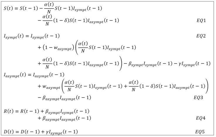
Where Isympt(t) – respectively Iasympt(t) – corresponds to the number of symptomatic (respectively asymptomatic) individuals on the date t with the following assumptions:
- The infection rate α(t) time dependent and associated with symptomatic individuals is reduced by the factor δ in the process of contamination induced by an asymptomatic patient (see EQ1 and EQ2). This parameter is estimated but its initial value is set at 50% as proposed in the study [2] carried out by the Imperial College COVID-19 Response Team.
- The recovery rate βsympt and βasympt are differentiated between symptomatic and asymptomatic cases (see EQ4). Their inverse represents the average recovery time of an infected patient.
- The case-fatality rate ϒ is only associated with symptomatic individuals. Since an asymptomatic individual does not die from COVID-19, the only possible exit from this state of contamination is recovery (see EQ5).
- New infections induced by symptomatic and asymptomatic individuals are distributed according to the weighting factor wasympt (see EQ2 and EQ3)
To improve the model goodness of fit and to take into account lockdowns, the infection rate α(t) is supposed to be time-dependent.
Noting Tconf the date on which the lockdown began, the infection rate is assumed to follow the exponential decrease below:

Where the parameter Kante (respectively Kpost) corresponds to the decay rate ante (respectively post) lockdown. The decay rates are assumed to be proportional:
Kpost = h x Kante
The adjustment factor h is not integrated into the calibration process and is fixed upstream by means of a dedicated study (see the calibration section below). The elements Kante and α(0) are estimated within the calibration process.
SIRD Model Calibration Methodology
The estimation technique considered in this study is based on the following optimization program:
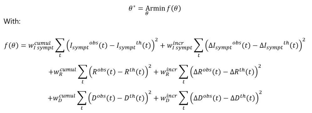
And where θ = (α(0),Kante,δ,βsympt,βasympt,ϒ) represents the vector of parameters to be estimated.
The target function corresponds to the squared differences between the observed and theoretical numbers, in cumulative and incremental vision. Since asymptomatic cases are not observed in practice, the calibration process focuses on the different observable quantities (i.e. numbers of symptomatic cases, deaths, recoveries).
The following elements corresponds to the weights associated with each of the components of the target function:

Further investigation areas
How to measure the effect of lockdowns?
Having an epidemiological model making short and medium-term projections can be particularly useful to help measuring the effects of lockdowns. This can enable public authorities to compare the number of people infected with the capacities of health care units and in particular intensive care units. Readers may consult the study by Massonnaud and al. [3] on the subject.
Note that the infection rate α(t) is homogeneous to the product of a probability of contamination with an average number of individuals encountered by an infected person at each unit of time. Various research papers have made assumptions about contact reduction rates in the implementation of lockdowns. In Di Domenico and al [4], several INSERM researchers report, in particular, reduction rates of 80% – 73% and 90% respectively – following the implementation of lockdowns in France – respectively in the United Kingdom and Shanghai respectively).
Noting τ the contact reduction rate and D the duration of the pandemic episode (calculated, for example, over time periods weighted by the number of incremental deaths observed at each date), it is possible to write:
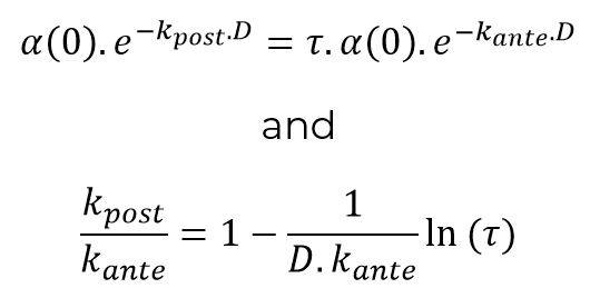
This relation makes it possible to objectify the parameter h introduced above from the relationship:

For a duration of 40 days, consistent with the orders of magnitude observed for COVID-19 events in China and South Korea, and a speed of convergence Kante of approximately 0.2%, the parameter h is homogeneous to a factor 20.
Adjusting the speed parameters Kante and Kpost makes it possible to report on the impact of lockdowns.
Stochastic adaptation of the SIRD model
Epidemiological models, in their most standard use, are projected in a deterministic way. However, projections are particularly sensitive to the robustness of the parameters considered (source of variability generally referred to as “estimation error”) and even in some cases to sampling errors associated with the projection of the model’s compartments.
Various techniques can be used to quantify the estimation error, such as a boostrap methodology applied to the underlying databases or the specification of distribution laws associated with the observations in order to characterize the maximum likelihood estimator law of the SIRD parameters.
In order to take into account sampling errors, it is possible with a sufficient sample to use a “central limit theorem” type approach and to deduce a simulation method from it.
For example, to generate the sampling fluctuations associated with the deaths compartment, the following variable could be considered:
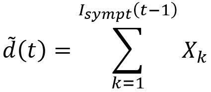
Where ᵭ(t) is the random variable for the number of deaths during the period t and (Xk)k a family of independent and identically distributed laws according to Bernoulli’s law of probability equal to the case-fatality rate ϒ.
The implementation of the central limit theorem leads to the following approximation for drawing the number of deaths in the period t:

The construction of the random variables associated with the other states of the SIRD model (i.e. symptomatic and asymptomatic recovered cases, new infections, etc.) is based on similar approaches.
These different techniques provide a framework for the results derived from deterministic projections.
Part 2. Calibration of the model on French COVID-19 data
The parameters of the SIRD model presented previously were calibrated on the French COVID-19 data, for the period between 01/23/2020 and 04/26/2020[1]. These data were reprocessed using the methodologies detailed in the first part to incorporate proportions of asymptomatic individuals in the contaminated and recovered populations.
The model was also back tested on the data between 04/26/2020 and 05/04/2020, when the study was carried out.
Fitting the SIRD model to the data
Due to the large number of parameters to be estimated, it is essential to have relevant values available for the calibration process initialization.
The orders of magnitude of the various model parameters were discussed in the previous note on standard SIRD modelling [1]. However, it should be noted that in this study the proportion of wasympt of asymptomatic individuals has been set at 20%, in accordance with the latest estimates published by the medical research community. The initial values of the recovery rates for symptomatic and asymptomatic individuals were 7% and 20% respectively, consistent with recovery times of 14 and 5 days respectively (incubation times frequently highlighted by medical research).
The values of the estimated parameters are shown in the table below:
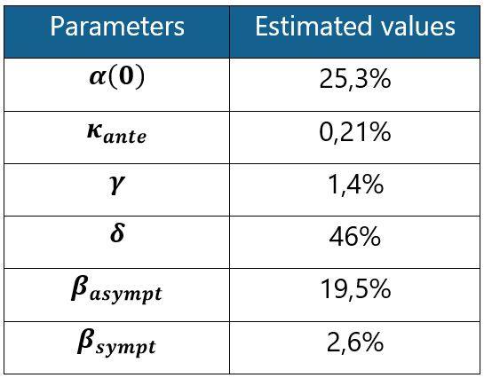
Table 1: SIRD model parameter estimates based on French data
The graphs below show the adjustment of the theoretical populations induced by the SIRD model on the observed target data.
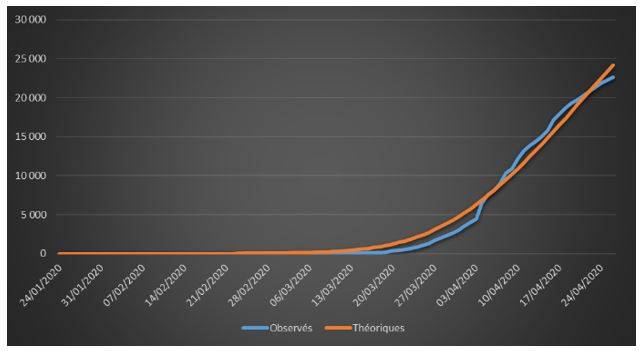
Figure 1: Cumulative observed and theoretical deaths on French data (01/24/2020 – 04/26/2020)
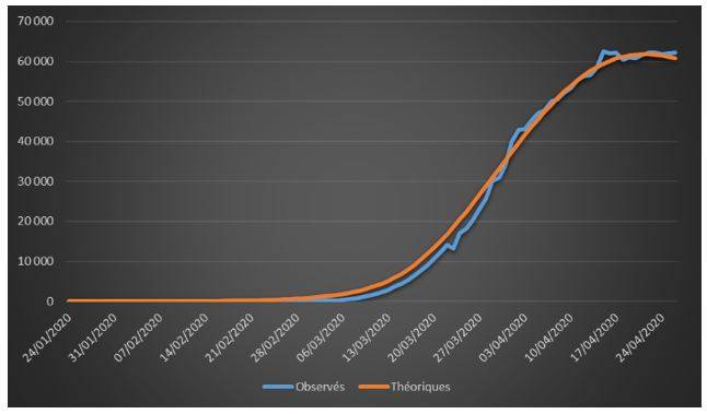
Figure 2: Cumulative observed and theoretical confirmed cases on French data (01/24/2020 – 04/26/2020)
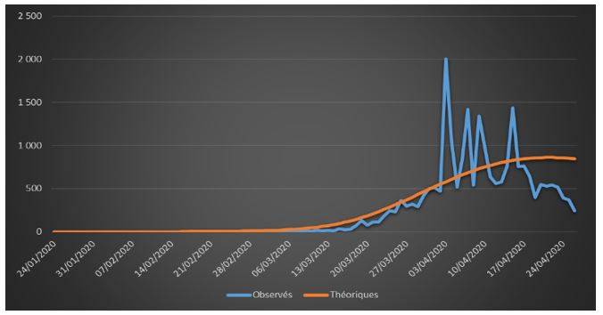
Figure 3: Observed and theoretical incremental deaths on French data (01/24/2020 – 04/26/2020)
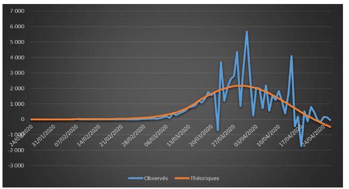
Figure 4: Observed and theoretical incremental confirmed cases on French data (01/24/2020 – 04/26/2020)
The adjustments are globally satisfactory. The deaths projected by the model seem nevertheless higher than the observed deaths. This phenomenon is due to relatively high estimate of the case-fatality rate (ϒ around 1.4%). We will come back to this issue in the rest of the study.
Backtesting of the SIRD model
The backtesting of the SIRD model over the period between 04/26/2020 and 05/04/2020 leads to the results presented in the table below:

Table 2: Comparison of the number of symptomatic cases and deaths as of 05/04/2020
The number of infected people projected by the model is lower than observed. This can be explained in particular by the calibration process which relies on the ante and post lockdown data. Indeed, even if the model makes it possible to cover these two periods based on a specific parametrization of the infection rate, the distortion of the underlying risk remains difficult to capture. Moreover, the projected number of deaths is higher than the observed number. This is due to the level of the estimated case-fatality rate, which is relatively high, although in line with the orders of magnitude that emerge in experts publications.
The values of the reproduction number R0 estimated on the observed and theoretical data are very close and equal to 1.1 [1]. These relatively low levels are due to the fact that the estimate is based on both ante and post lockdown data. The R0 post lockdown are significantly lower with values of 0.5 and 0.4 respectively on observed and theoretical data. Recall that when the level of R0 is less than 1, the epidemic is gradually dying out and on the contrary, it is bound to spread. Note that in our previous post [1], the R0 measured on the first epidemic stage before lockdown was up to 2.93. This parameter is proportional to the infection rate, itself proportional to the number of possible contacts in the population. As lockdown induces a reduction of 80% of contacts (see section “How to measure the effects of lockdowns”), it leads to an adjusted value of 0.6% homogeneous with the estimates of R0 after lockdown presented above.
SIRD model projection
As mentioned above, the estimated case-fatality rate appears to be relatively high following the backtesting results. An additional estimate of this parameter in order to converge the number of deaths observed and projected returns a value of 0.4% for this parameter.
The graphs below show the patterns of deaths and symptomatic infections projected on 2020.
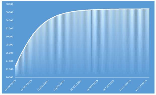
Figure 5: Cumulative number of deaths of COVID-19 projected in 2020 on French population
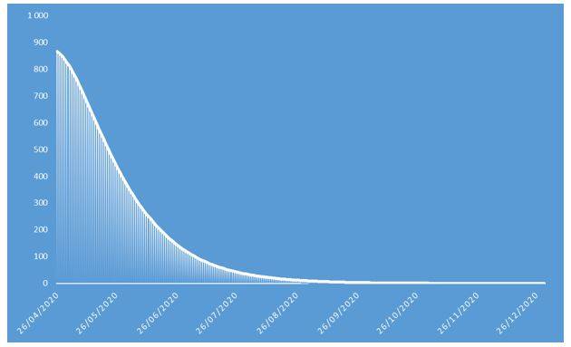
Figure 6: Number of incremental deaths of COVID-19 projected in 2020 on French population
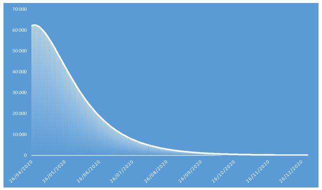
Figure 7: Number of COVID-19 contaminations projected in 2020 on French population
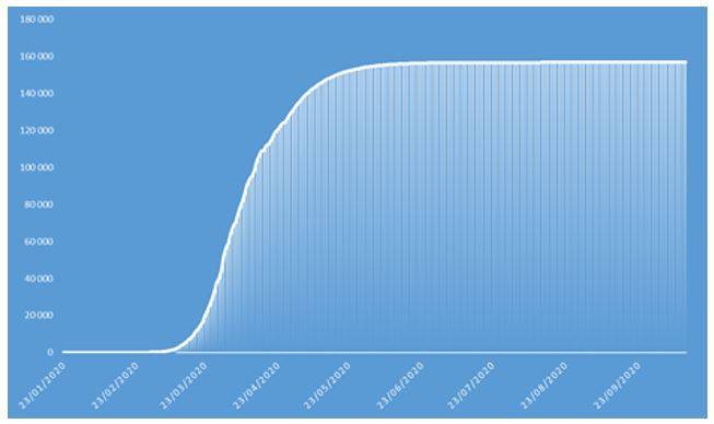
Figure 8: Cumulative number of confirmed COVID-19 cases projected in 2020 on French population
These projections were made conditional on the health situation on May 4, 2020, date of the study. Therefore, they may gradually deviate from the observations, particularly following the relieved lockdown policy of May 11, 2020, which will have an effect on the distortion of the risk and on the parameters governing the pandemic dynamics.
These projections identify an epidemic peak at the end of April 2020 and an overall number of deaths caused by COVID-19 of approximately 37.000 in the French population in 2020. The overall number of symptomatic contaminations amounts to about 162.000 cases, corresponding to the ceiling shown in Figure 8.
To go further…
The SIRD model presented in this study provides projections of the different compartments considered (susceptible, symptomatic and asymptomatic contaminated, recovered, deaths) over a short and medium term horizon.
Further studies could allow us to construct a stochastic approach around this deterministic model and make adjustments to the parameters after estimation. It is thus possible to simulate scenarios of lockdowns and relief of it by successively adjusting the contagion rate which can be considered proportional to the number of contacts observed in a population. Similarly, an improvement in medical treatments of COVID-19 could be reflected by consistently adjusting the model’s case-fatality or recovery rates.
These processing methods make it easy to calculate the sensitivity of the SIRD model to potential changes in the health context, which can be compared with available information on the capacities of health care units in a geographical area of interest. In particular, it enables the anticipation of the pandemic risk in the medium term by evaluating its health and economic impacts. Nevertheless, it is crucial to note the high sensitivity of the results obtained to the structure of the model and its parameterization, all the more so as the expert opinion that allows us to specify certain hypotheses may still evolve considerably with the progress of medical research on COVID-19 in the coming months.
Learn more about COVID-19 : Epidemioligical models & calibration issues
Marielle de la Salle, Head of addactis Lab
[1] Epidemiological models and calibration issues on COVID-19 data – addactis® note, April 2020
[2] Imperial College COVID-19 Response Team, Impact of non-pharmaceutical interventions to reduce COVID-19 mortality and healthcare demand, March 2020
[3] Massonnaud et al., COVID-19: Forecasting short term hospital needs in France, March 2020
[4] Di Domenico et al., Impact attendu du confinement en Île-de-France et stratégies de sortie possibles, April 2020

